— August 6, 2018
You are probably ending your A/B tests either too early or too late.
The standard best practice in the conversion optimization industry is to wait until two conditions have been met before ending an A/B test. First, that a representative sample is obtained. Second, that the winner of the test can be declared with 95% certainty or greater. You can see the latter standard touted here and here and here.
So why is it that Jeff Bezos writes this in an annual letter to shareholders?
“Most decisions should probably be made with somewhere around 70% of the information you wish you had. If you wait for 90%, in most cases, you’re probably being slow.”
Notice he is not laying down an immutable law; he says ‘most.’ Still, what is the dynamic he is describing?
It is opportunity cost. There is a cost to not acting on the information you have and instead opting to wait for greater certainty, but we rarely make a robust effort to calculate that opportunity cost and compare it to the potential gains of continued testing.
A hypothetical
Let’s take a hypothetical example. These are the results of an A/B test for the lead generation page of high-ticket-value product – perhaps a SaaS company. The test has been running for two months.
| A | B | |
| Visitors | 1,000 | 1,000 |
| Conversions | 100 | 120 |
Right now there is an 8% probability that we would have seen these or more extreme results in B’s favor if B was inferior to or equal to A. Let’s see an approximation of what the probability curves look like in this situation.

Figure 1
If we continue the test, and if we assume that the data keeps coming in the same proportions, it would take roughly three weeks to get to statistical significance. (Of course, if B’s advantage grows or shrinks the time to significance could shorten or lengthen.)
What are we losing during that time?
If we discontinue the test today then as best as we can guess, we would gain a lift that would give us an average of a 2% higher conversion rate – except that half the visitors are already seeing option B, so it’s likely to be closer to 1%. Still, in absolute terms, we would be gaining an average of about 7 or 8 more leads than we would otherwise over three weeks – a number that would likely be significant to a sales team.
Of course, there is also an 8% probability that A is actually the superior choice. But not only does 8% represent roughly just a 1 in 12 chance, look at where the pink area in the graph above is falling. The scale of the potential loss 8% of the time – the widest likely gap between a leading A and a trailing B – is about 2%, while the scale of the potential gain 92% of the time – the widest likely gap between a leading B and a trailing A – is about 6%. When you take into account the effect of these outcomes, the probabilistic value of choosing B increases.
It’s perhaps obvious, but still worth noting that waiting for significance is not the same thing as waiting for certainty. Three weeks later we would still have a 5% chance of making the wrong pick – there would still be a pink overlap area.
95% is just a convention
So why is it that 95% became a standard for statistical significance? In a normal data distribution, 95% is two standard deviations from the mean (a deviation being a measure of dispersion.) Apart from that, there is nothing special about 95%; it is just a convention.
Certainly, a convention is necessary. The probability curves in the graph above never actually touch the axis, but slope towards it until they touch zero on one end and the maximum on the other. What the 95% convention allows us to do is quickly define how widely dispersed the curves are. We can say, “95% of the time, our sample results will fall within x% of the actual results in the total population.” This, in effect, slices the bell curves on their outward slopes so their width can be measured in a standardized way.
This convention also provides a standard for academics to report their results: they can say, “these results are significant” or “these results are not significant.” This makes reports easier to understand and sum up.
But other than these communicative advantages, there is nothing magical about 95%.
When to end an A/B Test
First, let’s not forget the need for a representative sample. It’s best to only check your test on the same day of the week that you started it, so that each monitoring is comprised of complete weekly cycles.
However, we can confidently make these two statements:
- In any A/B test that has been running for a reasonable time there is a cost to not presently concluding a test and choosing the version which the data tells you is superior: this is the opportunity cost.
- There is also a cost to ending a test and perhaps making the wrong choice: this is the error cost (and, of course, it is present even at 95% significance.)
Rather than using the somewhat arbitrary 95% criterion, a better guideline for ending an A/B test is when the opportunity costs start becoming greater than the error costs.
In collaboration with Santa Clara-based data scientist, Wesley Engers, my company has created an Excel document that tells you when you have crossed this inflection point. You can download it for free here.
How to Use the Calculator
Here is what you put in to the calculator, and here are the most important outputs:
| Inputs | Outputs |
|
|
The first five items in the input column are fairly self-explanatory, but the sixth might need some elaboration.
In order to calculate what the error costs are we need to project them over a certain period of time from the beginning of a test; we are calling this the Amortization Period. This is the time over which the results of the test are likely to be useful to you.
Given the number of elements that might change in both the page you are testing and your business situation – product line updates, customer preferences, interaction with other on-page elements, etc. – we recommend setting the Amortization Period to 534 days (which comes to 18 months.) However, if you anticipate a complete site re-design in a few months time, then by all means use a smaller number of days for this field. Likewise, if you foresee your situation as fairly stable, then you might want to switch to a longer Amortization Period.
The outputs include the estimated lift of the currently superior version, the P-Value so far (which is easily translatable to a confidence percentage,) and the conclusion of the model to the question: Are prospective opportunity costs greater than prospective gains in accuracy?
The answer to this question is not meant to be a decision-making machine, replacing the arbitrary 95% criterion. Yes, you should make your decision based on ROI rather than arbitrary rules, but there are multiple other considerations affecting your investment and returns that you will want to take into account. Here are just a couple of them:
- This calculator only takes into account returns for this experiment. If you are planning on conducting other experiments, which potentially might bear fruit, continuing your current experiment also delays their returns. This favors a quicker conclusion to the experiment.
- On the other hand, we often do not calculate the cost for preparing a new A/B. If this model is pushing you towards quicker iterations, remember your time is a cost too. This favors a slower experimental tempo. (You can read about some other ROI considerations here.)
With this or any other decision-making methodology, often the toughest call is when the test is not giving you a clear answer. If you have collected a sizable sample and the result is still too close to call – both in terms of p-value and opportunity/error costs – often the best course of action is to choose a winner before it is declared by the models and look for another testing opportunity that might provide you with greater returns.
How the Calculations are Made
If you would like to know what is under the hood of the calculator, following is an explanation.
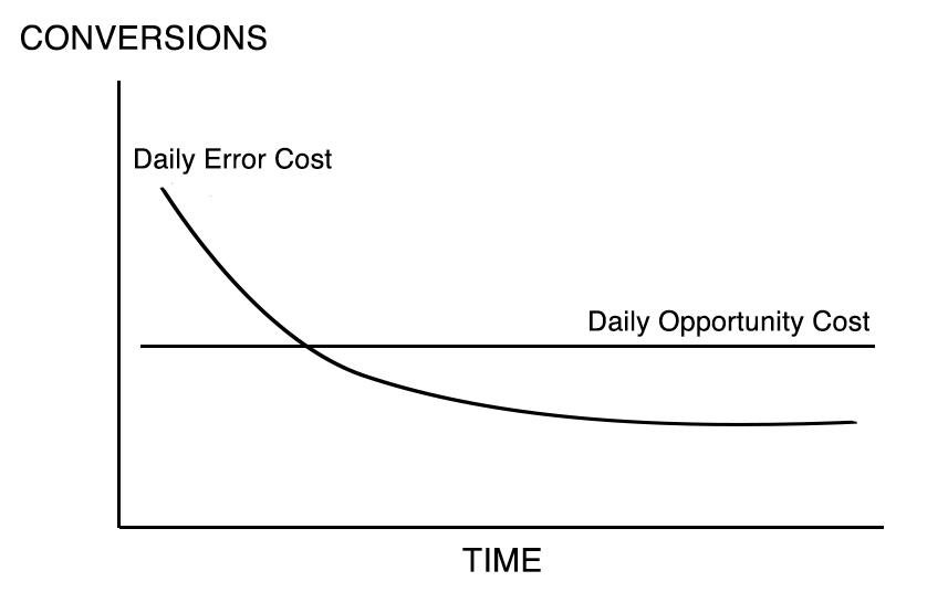
Figure 2
The first things we calculate are the Average Number of Daily Lost Conversions from Not Ending an Experiment (Daily Opportunity Cost) versus Average Number of Daily Lost Conversions from Making the Wrong Choice (Daily Error Cost.) In real life, these lines would go up and down in response to random fluctuations of the data, but if we assumed that it arrived consistently in the same proportions, the lines would look something like this.
The Daily Error Cost line is sloping down because as the data is gathered, statistical confidence is gained, and the chances of error decrease. The Daily Opportunity Cost line is flat because, as mentioned, we are assuming that the results are not fluctuating: if the results for each version don’t vary, neither will the average daily cost of not choosing a winner.
How do we calculate these numbers? Daily Opportunity Cost is just the difference between the number of conversions of the better-performing version with the number of conversions of the worse-performing version, divided by the number of days the test has been running and then divided by two, since half the visitors are already seeing the superior version.
Daily Error Cost is a more complicated statistical calculation that you can review in the excel sheet, but here is Wesley’s summary. (Don’t be discouraged… it gets much easier after this.)
Daily Error Cost is calculated by determining how many conversions would be lost if the wrong choice of version was made. For example, if the current higher conversion is version A but the truth is actually that version B has a better conversion rate then the estimated number of lost conversions is calculated for using version A instead of the correct version B. Mathematically, this is done by calculating the estimated difference is conversion rates assuming that version B is actually better. This is based on the normal distribution of the difference between the conversion rates of version A and version B. Mathematically, first let’s suppose that PA> PB then this is the expected value of PA – PB given that PA – PB <0 (i.e. E[PA – PB| PA – PB <0]). This can be calculated by doing the integral from -1 to 0 of x*p(x) where p (x) is the density function of the normal distribution with mean PA – PB and standard deviation.

See Data Value tab in Excel sheet for calculation.
Now let’s assume that we are at a certain point in the life of the test, and we are considering ending the test today or tomorrow. In Figure 3, we see the case where we discontinue the test today. We are accepting the Daily Error Cost over the remaining Term of Amortization. In Figure 4 we see the case where we continue the test until tomorrow, accepting the Opportunity Cost over that period, then switch to the lower Error Cost.
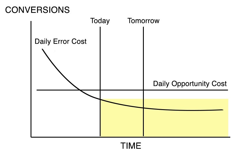
Figure 3 |
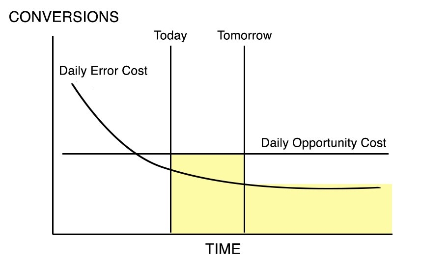
Figure 4 |
Notice that we are adding an area and losing an area in Figure 4. Figure 5 makes this clearer.
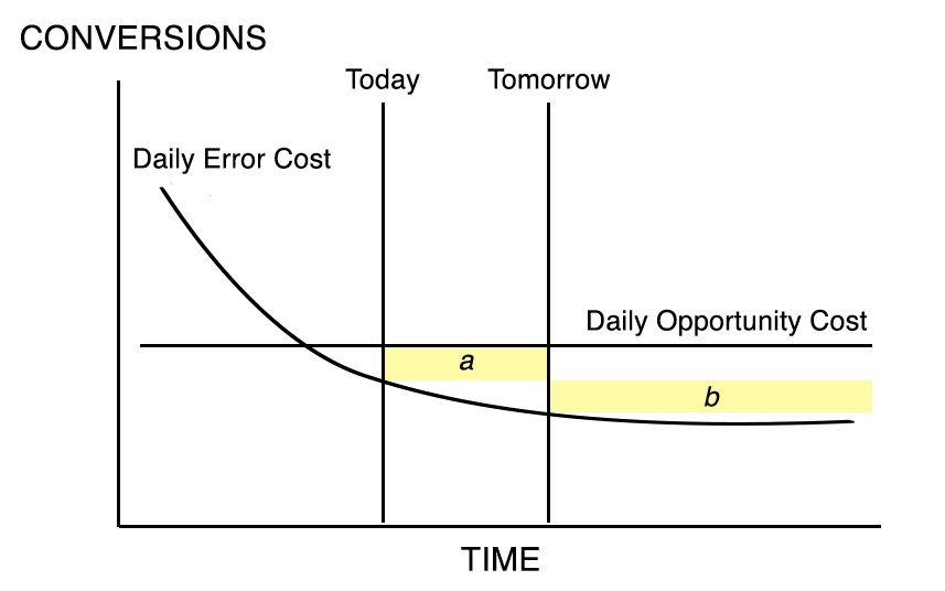
Figure 5
When we choose to continue the test, we are adding Area a but losing Area b.
If we are taking away more than we are adding – that is, if Area b is larger than Area a, then the Error Costs we are losing will be greater than the Opportunity Costs we are acquiring. It makes sense to continue the experiment.
However, if we are adding more than we are taking away, if Area a is larger than Area b, then the Opportunity Costs we are paying to continue the experiment will be larger than the Error Costs we are losing with a more accurate data sample. We should discontinue the experiment.
It’s clear then that the Optimum Time to discontinue the experiment would be when Area a starts becoming greater than or equal to Area b, because that will result in increasing costs.
Calculating these areas for tomorrow is fairly easy. Area a is a breadth by length calculation:
(Daily Opportunity Cost – Daily Error Cost) x 1 day since it’s tomorrow
Area b is calculated by projecting data one day into to future, so as to estimate the Daily Decrease in Error Cost, then multiplying it by the remaining days in the Amortization Term:
Decrease in Error Cost x (Term of Amortization – Days Test Has Been Conducted – 1 since it’s tomorrow)
When Area a is greater than or equal to Area b, then the Opportunity Costs start accruing faster than the Error Costs. This is when you should consider discontinuing the test. In the hypothetical case of the SaaS company that we started this article with, the model recommends concluding the test, even though our confidence level is below 95%.
Conclusion
As we’ve mentioned, this article is not intended to replace one hard-and-fast rule (“End your A/B tests when you have 95% significance!”) with another. It is to make these points:
- We need to take into account the opportunity cost of not presently ending an A/B test
- We should arm ourselves with tools to calculate these opportunity costs and compare them with error costs
- Marketers cannot afford to think as academics do, searching for Truth (with a capital T.) Our job is to provide the best ROI, and that might mean operating with less certainty than we would like.
This model might push people who receive a lot of data past the point of 95% confidence. However, I imagine it will be most useful for marketers whose data comes in slowly. The model will give them leave to terminate experiments before they reach statistical significance. Often times, marketers with little data are discouraged from A/B testing because of the 95% shibboleth, and are instead urged to follow ‘best practices.’
That is a disservice. In the real world, if something is 5 or 10 times likelier to be true than not, that is significant; 19x (what 95% translates to) is not a mystical threshold.
Special thanks to Georgi Georgiev from Analytics Toolkit for comments and reviewing statistical methodology in this article.
Business & Finance Articles on Business 2 Community
(122)
Report Post


